
The recommended way to use dragmapr is to treat a layout as an
editable composition object – a
dragmapr_state – and carry it through three steps:
compute  ->  compose  ->  render
(layout)     (edit)       (static / interactive)
The state is plain, reproducible data: region and label offsets (as
metre deltas), the projected crs, a
geometry_id, the selected_feature, and a
monotonically increasing version. Because the geometry and
the editorial state are kept separate, you can recompute the layout
while preserving manual edits, and the same state object drives
the interactive editor, the static renderer, and any persistence.
The older route – exporting offset CSVs and calling
as_dragmapr() – still works, but it is now the low-level
escape hatch rather than the main road.
1. Compute
In a full pipeline the layout comes from explodemap, which computes a mathematically valid exploded layout and hands it over as a state:
library(explodemap)

layout <- explode_grouped(my_sf, region_col = "region")
state  <- as_dragmapr_state(layout)   # dx_m/dy_m deltas + crs + geometry_id
For a self-contained example we build the equivalent state directly, so this vignette runs with only dragmapr installed:
library(dragmapr)

make_square <- function(x0, y0, size = 100000) {
  sf::st_polygon(list(rbind(
    c(x0, y0), c(x0 + size, y0), c(x0 + size, y0 + size),
    c(x0, y0 + size), c(x0, y0)
  )))
}

regions <- sf::st_sf(
  region = c("North", "South", "East", "West"),
  geometry = sf::st_sfc(
    make_square(0, 140000), make_square(0, 0),
    make_square(140000, 70000), make_square(-140000, 70000),
    crs = 3857
  )
)

state <- d_state(
  region_offsets = data.frame(
    region = c("North", "South", "East", "West"),
    dx_m   = c(0, 0, 60000, -60000),
    dy_m   = c(50000, -50000, 0, 0)
  ),
  crs = 3857,
  geometry_id = "synthetic-quad-v1"
)
state
#> $level
#> [1] "region"
#>
#> $region_offsets
#>   region   dx_m   dy_m
#> 1  North      0  50000
#> 2  South      0 -50000
#> 3   East  60000      0
#> 4   West -60000      0
#>
#> $label_offsets
#> [1] label_id region   dx_m     dy_m
#> <0 rows> (or 0-length row.names)
#>
#> $expanded_groups
#> character(0)
#>
#> $view
#> NULL
#>
#> $version
#> [1] 0
#>
#> $crs
#> [1] 3857
#>
#> $geometry_id
#> [1] "synthetic-quad-v1"
#>
#> $selected_feature
#> NULL
#>
#> $styles
#> [1] region        fill          stroke        stroke_width  opacity
#> [6] label_visible highlight
#> <0 rows> (or 0-length row.names)
#>
#> $region_col
#> [1] "region"
#>
#> $label_id_col
#> [1] "label_id"
#>
#> $binding
#> $binding$region_col
#> [1] "region"
#>
#> $binding$label_id_col
#> [1] "label_id"
#>
#>
#> $schema_version
#> [1] "1.2.0"
#>
#> $package_version
#> [1] "0.3.1"
#>
#> attr(,"class")
#> [1] "dragmapr_state"
2. Compose
d_edit() is the friendly front door to the interactive
editor. It accepts a projected sf, an explodemap
grouped_exploded_map, or a dragmapr_layout,
seeded with the state:
d_edit(regions, region_col = "region", state = state)Inside Shiny, the widget reports every edit through an input named
paste0(outputId, "_state"). Rebuild a
dragmapr_state from it with d_widget_state()
so the server always holds the live composition:
output$map <- renderDragmapr(d_edit(regions, "region", state = state))

observeEvent(input$map_state, {
  state <- d_widget_state(input$map_state)
})

# Push a selection from R back into the browser:
updateDragmapr(session, "map", selected_feature = "East")
3. Render
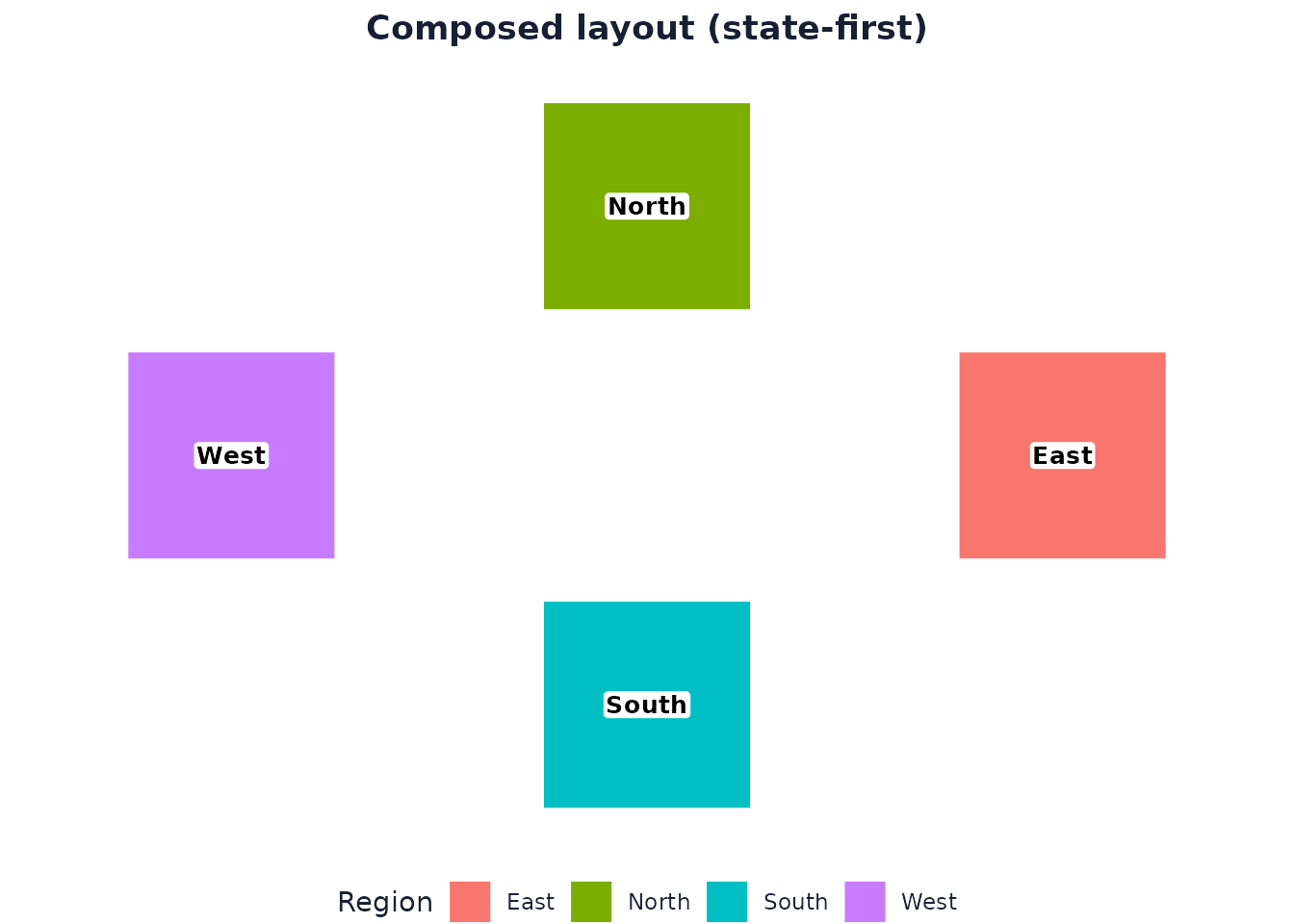
Because the state is just data, you can persist it and reproduce the
layout as a static ggplot2 image at any time – no browser
session and no recomputation:
path <- tempfile(fileext = ".json")
write_dragmapr_state(state, path)
state2 <- read_dragmapr_state(path)

render_dragged_map(
  regions,
  region_col = "region",
  state = state2,
  title = "Composed layout (state-first)"
)
The state object
A dragmapr_state carries:
-
region_offsets/label_offsets– metre deltas (dx_m,dy_m) keyed by a stable join key; -
crs– the projected CRS the deltas are expressed in (EPSG or WKT), so a saved state is safe to reapply later; -
geometry_id– a provenance tag for the geometry the state was composed against; -
selected_feature,expanded_groups,view– editor/dashboard state; -
version– a revision that bumps monotonically as edits accumulate.
The full lifecycle (validate_, merge_,
snapshot_/restore_,
inherit_drag_offsets(),
collapse_drag_offsets(), and JSON
read_/write_) operates on this object. A small
app can keep one canonical state, one draft state, and compare them
before enabling save/export:
canonical <- reactiveVal(state)
draft <- reactiveVal(state)

observeEvent(input$map_state, {
  draft(d_widget_state(input$map_state))
})

output$dirty <- renderText({
  changed <- !d_state_equal(
    draft(),
    canonical(),
    compare = "composition"
  )

  if (changed) "Unsaved layout edits" else "Layout saved"
})

observeEvent(input$save_layout, {
  validate_dragmapr_state(draft())
  write_dragmapr_state(draft(), "composition.json")
  canonical(draft())
})
When a workflow starts in explodemap, the handoff stays
the same: compute the layout, convert it once to a
dragmapr_state, edit the state, then render from the same
state.
library(explodemap)
library(dragmapr)

layout <- explode_grouped(my_sf, region_col = "region", plot = FALSE)
state <- as_dragmapr_state(layout, geometry_id = "service-territory-v1")

edited <- d_edit(layout, state = state)

render_dragged_map(
  layout$sf_grouped,
  region_col = "region",
  state = state,
  file = "edited-layout.png"
)