Getting started with dragmapr

dragmapr is built around a deliberately small loop for draggable plots:

Start with projected sf geometry and a grouping column.
Open the draggable browser helper with drag_map_prototype(open = interactive()).
Drag regions, labels, or annotation boxes until the layout looks right.
Copy or download the offset CSVs from the helper panel.
Optionally reproduce the layout as a static ggplot2 image with render_dragged_map().

The interactive helper is the primary deliverable. Step 5 is optional — use it when you need a reproducible image for a report or publication.

Toy geometry

All examples below use a projected toy dataset so the workflow can be tested without downloading shapefiles.

library(dragmapr)

make_square <- function(x0, y0, size = 100000) {
  sf::st_polygon(list(rbind(
    c(x0, y0), c(x0 + size, y0), c(x0 + size, y0 + size),
    c(x0, y0 + size), c(x0, y0)
  )))
}

regions <- sf::st_sf(
  region = c("North", "South", "East", "West"),
  label  = c("North", "South", "East", "West"),
  geometry = sf::st_sfc(
    make_square(0,       140000),
    make_square(0,            0),
    make_square( 140000,  70000),
    make_square(-140000,  70000),
    crs = 3857
  )
)

`drag_map_prototype()` — full parameter reference

Data

These three arguments identify the geometry and what to group or label.

Argument	Default	Description
`x`	(required)	Projected `sf` object. Must not be in a geographic (lon/lat) CRS.
`region_col`	(required)	Column name that defines draggable groups.
`label_col`	`region_col`	Column used for label text. Defaults to the grouping column.

# Minimal call — one grouping column used for both groups and labels
drag_map_prototype(regions, region_col = "region", open = interactive())

# Separate column for label text
drag_map_prototype(regions, region_col = "region", label_col = "label", open = interactive())

Labels

Control whether labels appear and whether they can be dragged independently.

Argument	Default	Description
`labels`	`TRUE`	`TRUE` derives one label per region automatically. `FALSE` shows no labels. Supply a data frame from `as_drag_labels()` or `as_drag_annotations()` for custom labels.
`draggable_labels`	`TRUE`	When `TRUE`, labels can be moved independently. When `FALSE`, labels follow their region but cannot be repositioned on their own.

# No labels
drag_map_prototype(regions, region_col = "region", labels = FALSE, open = interactive())

# Labels follow regions but cannot be dragged separately
drag_map_prototype(regions, region_col = "region",
                   draggable_labels = FALSE, open = interactive())

# Custom label data frame
custom_labels <- make_region_labels(regions, region_col = "region", label_col = "label")
drag_map_prototype(regions, region_col = "region",
                   labels = custom_labels, open = interactive())

Label styling

Choose between three marker shapes for short text labels — rounded box, circle, or text-only — and control their sizes and font.

Argument	Default	Description
`label_marker`	`TRUE`	Draw a visible marker shape behind label text. `FALSE` is a shortcut for `label_marker_shape = "none"`.
`label_marker_shape`	`"rect"`	Shape behind the label text: `"rect"` (rounded box), `"circle"`, or `"none"` (text only with an invisible drag target).
`label_text_size`	`11`	Label text size in browser pixels. Applies to all label types.
`label_width`	`64`	Width of rounded-box label markers in pixels.
`label_height`	`30`	Height of rounded-box label markers in pixels.
`label_radius`	`12`	Circle radius in pixels. Used when `label_marker_shape = "circle"`.
`label_box_width`	`150`	Width of draggable annotation box (info-box style) in pixels.
`label_box_height`	`72`	Height of draggable annotation box in pixels.

# Rounded-box markers (default) — adjust size and text
drag_map_prototype(
  regions, region_col = "region",
  label_marker_shape = "rect",
  label_text_size    = 12,
  label_width        = 80,
  label_height       = 32,
  open = interactive()
)

# Circle markers
drag_map_prototype(
  regions, region_col = "region",
  label_marker_shape = "circle",
  label_radius       = 18,
  label_text_size    = 11,
  open = interactive()
)

# Text only — no visible marker, just draggable text
drag_map_prototype(
  regions, region_col = "region",
  label_marker_shape = "none",
  label_text_size    = 13,
  open = interactive()
)

# Annotation boxes (info-box style with connectors)
notes <- as_drag_annotations(
  make_region_labels(regions, region_col = "region"),
  width_px       = 160,
  height_px      = 70,
  connector      = TRUE,
  connector_type = "elbow"
)
drag_map_prototype(
  regions, region_col = "region",
  labels           = notes,
  label_box_width  = 160,
  label_box_height = 70,
  open = interactive()
)

Connectors

Connector lines link a label or annotation box back to its region anchor. They are only drawn for labels that have connector = TRUE in their label data frame — set that flag via as_drag_annotations(..., connector = TRUE) or as_drag_labels(). The line style ("straight", "elbow", "curve", "squiggle") is stored per-label in the connector_type column.

Argument	Default	Description
`connector_color`	`"#334155"`	Browser connector line colour.
`connector_linewidth`	`1.3`	Connector line thickness in browser pixels.
`connector_linetype`	`"solid"`	Browser connector line pattern: `"solid"`, `"dashed"`, or `"dotted"`.
`connector_endpoint`	`"none"`	Browser connector endpoint: `"none"` or `"arrow"`.
`connector_smart`	`FALSE`	Let the browser choose straight, elbow, or curved connector geometry from the current label displacement.

drag_map_prototype(
  regions, region_col = "region",
  labels              = notes,   # labels with connector = TRUE
  connector_color     = "#334155",
  connector_linewidth = 2,
  connector_linetype  = "dashed",
  connector_endpoint  = "arrow",
  connector_smart     = TRUE,
  open = interactive()
)

Movement context

Movement context is optional and off by default. It helps explain where a moved region came from without changing the underlying offset data.

Argument	Default	Description
`show_origin_outlines`	`FALSE`	Draw the original outline for regions with non-zero offsets.
`show_movement_connectors`	`FALSE`	Draw a line from each moved region’s original representative point to its current location.
`movement_connector_color`	`"#64748b"`	Movement connector colour.
`movement_connector_opacity`	`0.72`	Movement connector opacity from 0 to 1.
`movement_connector_linewidth`	`1.4`	Browser movement connector thickness in pixels.
`movement_connector_linetype`	`"solid"`	Movement connector pattern: `"solid"`, `"dashed"`, or `"dotted"`.
`movement_connector_endpoint`	`"closed"`	Movement connector endpoint: `"closed"`, `"open"`, or `"none"`.
`show_drag_trail`	`FALSE`	Browser-only fading outline trail while a region is actively dragged.

drag_map_prototype(
  regions, region_col = "region",
  show_origin_outlines = TRUE,
  show_movement_connectors = TRUE,
  movement_connector_color = "#64748b",
  movement_connector_linetype = "dashed",
  movement_connector_endpoint = "open",
  show_drag_trail = TRUE,
  open = interactive()
)

Static exports support origin outlines and movement connectors too:

render_dragged_map(
  regions,
  region_offsets = region_offsets,
  region_col = "region",
  show_origin_outlines = TRUE,
  show_movement_connectors = TRUE,
  movement_connector_linetype = "dotted",
  movement_connector_endpoint = "closed"
)

Initial positions

Supply previously exported offset tables to pre-load a saved layout so dragging can continue from where it left off.

Argument	Default	Description
`region_offsets`	`NULL`	Data frame with columns `region`, `dx_m`, `dy_m`. All regions start at zero when `NULL`.
`label_offsets`	`NULL`	Data frame with columns `label_id`, `region`, `dx_m`, `dy_m`. All labels start at zero when `NULL`.

# Resume from previously downloaded CSVs
region_csv <- read_offsets("drag_region_offsets.csv")
label_csv  <- read_label_state("drag_label_offsets.csv")

drag_map_prototype(
  regions, region_col = "region",
  region_offsets = region_csv,
  label_offsets  = label_csv,
  open = interactive()
)

read_label_offsets() is retained as an alias for read_label_state(), and apply_label_offsets() is retained as an alias for apply_label_state(). Likewise, make_labels() remains an alias for make_region_labels() for older scripts.

If the offsets were exported as a Spatial Studio project ZIP, use the one-line project renderer instead of wiring the CSV files together manually:

render_dragmapr_project(
  "dragmapr-project.zip",
  file = "dragged-map.png"
)

RStudio addin

In RStudio, install the package and use Addins > Launch dragmapr to open a compact prototype gadget. The addin looks for sf objects in .GlobalEnv, lets you choose the region and label columns, and assigns region_offsets and label_offsets when you click Done. Create or load the sf object before opening the addin. If you call dragmapr_addin() directly, pass env = to work with another environment.

Colour palette

Argument	Default	Description
`region_palette`	`NULL`	Named character vector mapping each region value to a hex colour string. Uses a built-in 8-colour cycling palette when `NULL`.

Matching the interactive palette to a render_dragged_map() call makes the draggable preview and the final static image look identical.

my_palette <- c(
  North = "#4C78A8",
  South = "#F58518",
  East  = "#54A24B",
  West  = "#B279A2"
)

drag_map_prototype(
  regions, region_col = "region",
  region_palette = my_palette,
  show_legend    = TRUE,
  open = interactive()
)

Legend

A compact colour legend can be embedded directly inside the browser helper. It is hidden by default because many maps are labelled and need no legend.

Argument	Default	Description
`show_legend`	`FALSE`	Show a colour legend in the helper.
`max_legend_keys`	`25`	Suppress the legend automatically when the number of groups exceeds this value. Set to `Inf` to always show it regardless of group count.
`legend_position`	`"bottom"`	Where the legend appears: `"bottom"`, `"top"`, `"left"`, `"right"`, or `"none"`.
`legend_title`	`"Region"`	Title shown above the legend keys.
`legend_values`	`NULL`	Optional character vector of region values to include in the legend. `NULL` includes all values.

drag_map_prototype(
  regions, region_col = "region",
  region_palette  = my_palette,
  show_legend     = TRUE,
  legend_position = "bottom",   # "top" | "left" | "right" | "none"
  legend_title    = "Region",
  legend_values   = c("North", "East"),
  max_legend_keys = 25,
  open = interactive()
)

Use label_values when an app should temporarily display only selected labels while preserving all label offsets:

drag_map_prototype(
  regions, region_col = "region",
  label_values = c("North", "East"),
  open = interactive()
)

Output file and display

Argument	Default	Description
`file`	`"drag-map.html"`	File path for the written standalone HTML.
`open`	`FALSE`	Open the file in the default browser via `browseURL()` after writing.
`side_panel`	`TRUE`	Show the built-in copy/download side panel. Shiny apps that provide their own export controls can set this to `FALSE` to reclaim the full canvas.
`map_background`	`"white"`	Helper background: `"white"`, `"transparent"`, `"light_grid"`, or `"dark"`.

# Write to a chosen path without opening (e.g. CI, server, or Shiny)
drag_map_prototype(
  regions, region_col = "region",
  file       = "output/my_map.html",
  map_background = "light_grid",
  side_panel = TRUE,
  open       = FALSE
)

# Embedded in a Shiny app — hide the panel; the app provides its own controls
drag_map_prototype(
  regions, region_col = "region",
  side_panel = FALSE,
  file       = tempfile(fileext = ".html")
)

Optional: Static rendering

When you need a reproducible ggplot2 image, pass the exported offset tables to render_dragged_map(). The data frames below stand in for downloaded CSVs:

region_offsets <- data.frame(
  region = c("North", "South", "East", "West"),
  dx_m   = c(0, 0,  60000, -60000),
  dy_m   = c(50000, -50000, 0, 0)
)

label_state <- data.frame(
  label_id = c("North", "South", "East", "West"),
  region   = c("North", "South", "East", "West"),
  dx_m     = c(0, 0,  25000, -25000),
  dy_m     = c(30000, -30000, 0, 0)
)

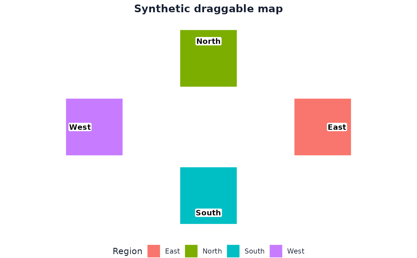
render_dragged_map(
  regions,
  region_offsets = region_offsets,
  region_col     = "region",
  label_col      = "label",
  label_offsets  = label_state,
  title          = "Synthetic draggable map"
)

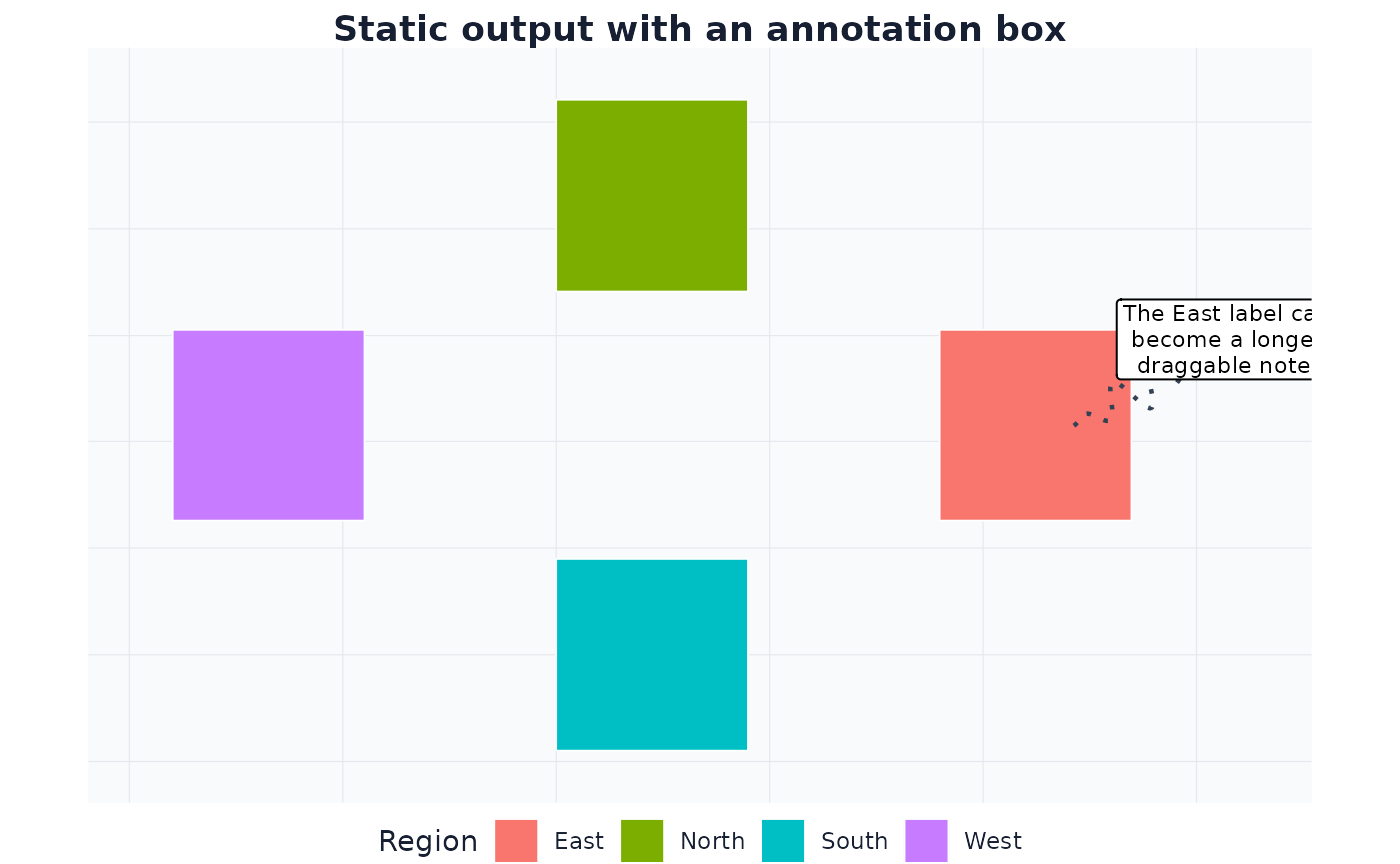
The same annotation types available in the interactive helper work in static output:

notes <- as_drag_annotations(data.frame(
  label_id = "east-note",
  region   = "East",
  label    = "The East label can become a longer draggable note.",
  x = 210000, y = 120000
), connector = TRUE, connector_type = "squiggle")

render_dragged_map(
  regions,
  region_offsets      = region_offsets,
  region_col          = "region",
  labels              = notes,
  label_offsets       = data.frame(
    label_id = "east-note", region = "East",
    dx_m = 80000, dy_m = 45000
  ),
  connector_linewidth = 0.8,
  connector_linetype  = "dotted",
  connector_endpoint  = "arrow",
  legend_title        = "Region",
  map_background      = "light_grid",
  title               = "Static output with an annotation box"
)

Edit the source features

Sometimes the right display map is not just a moved map. It is a lighter map: one or more features are removed, or a corrected feature is swapped in before the final layout is composed.

feature_rows <- spatial_feature_table(regions, key_col = "region")
feature_rows[, c(".feature_id", ".row", ".geometry_type")]

regions_without_north <- remove_spatial_features(
  regions,
  ids = "North",
  key_col = "region"
)

regions_only_south_west <- keep_spatial_features(
  regions,
  ids = c("South", "West"),
  key_col = "region"
)

The editing helpers return ordinary sf objects, so the result can go straight back into the draggable helper:

drag_map_prototype(
  regions_without_north,
  region_col = "region",
  open = interactive()
)

A small Shiny editor

This is the same loop inside a minimal Shiny app: render the widget, receive state from the browser, and push a live display update from the server.

library(shiny)
library(dragmapr)

ui <- fluidPage(
  checkboxInput("origin", "Show origin outlines", TRUE),
  dragmaprOutput("map", height = "650px"),
  verbatimTextOutput("state")
)

server <- function(input, output, session) {
  current_state <- reactiveVal(dragmapr_state(crs = 3857))

  output$map <- renderDragmapr({
    dragmapr_widget(
      regions,
      region_col = "region",
      state = current_state(),
      display_options = dragmapr_display_options(
        show_origin_outlines = isTRUE(input$origin)
      )
    )
  })

  observeEvent(input$map_state, {
    current_state(dragmapr_widget_state(input$map_state))
  })

  observeEvent(input$origin, {
    updateDragmapr(session, "map", show_origin_outlines = input$origin)
  })

  output$state <- renderPrint(summary(current_state()))
}

shinyApp(ui, server)

Working with your own data

Use projected polygon data for editing. If your source file is longitude and latitude, run it through prepare_dragmapr_sf() first so offsets are measured in metres:

my_sf <- read_dragmapr_sf_url("https://example.com/regions.geojson")
my_sf <- prepare_dragmapr_sf(my_sf)

drag_map_prototype(
  my_sf,
  region_col = "region_name",
  label_col = "short_name",
  map_background = "light_grid",
  open = interactive()
)

The package keeps the display edits separate from the source geometry. That separation is the useful part: you can drag, remove, restore, export, and render without hiding how the final map was made.